Semi Supervised Classification with Advesarial Auto Encoders¶

General Concept¶

In the concept described in [1], AAE can be submitted to semi-supervised learning, training them to predict the correct label using their latent feature representation, and based on a semi-supervised training set.

As described in the overview of this project, the adversarial autoencoder contains a simple AE at its center. The training method for semi-supervised learning exploits the generative description of the unlabeled data to improve the classification performance that would be obtained by using only the labeled data.

As in many cases, unlabeled data is more abundant and accessible. Using it as part of the adversarial AE learning, will help the encoding improve, alongside it producing better labeling.

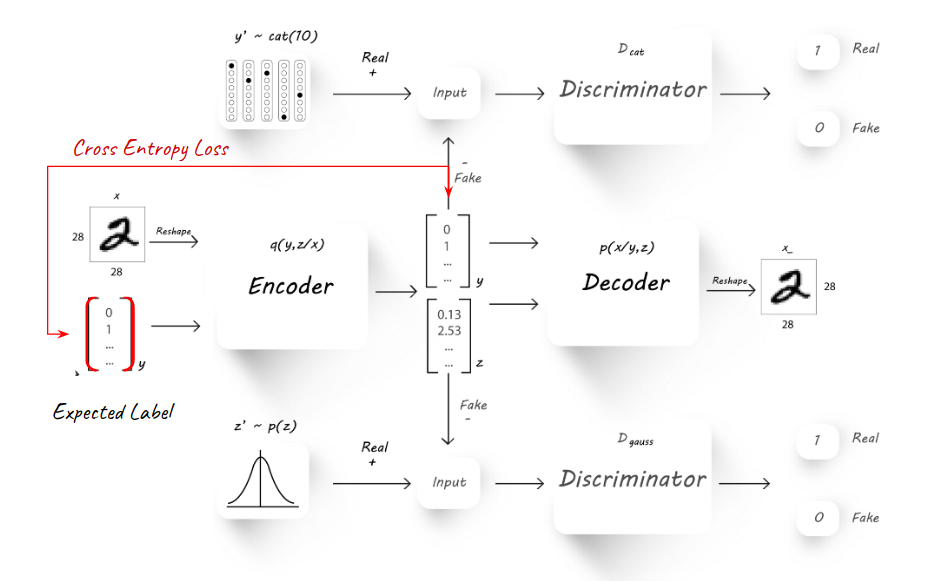
The general schema for semi-supervised learning can be seen here:

Inference and Perfomance Estimation¶

The basic schema follows the exact implementation of the AAE, with the only difference of introducing a labeled image from time to time into the training process. The labeled image is treated differently and is measured using a new Cross Entropy loss again the known target label. This loss only effect the Encoder (Q) - causing it to learn how to predict the labled images currectly over the latent y categorical part.

Followed the training process, the semi-supervised AAE is in fact a classifier as any other. The inference is performed using the decoder alone (Q) and observing the latent y part of the latent features, which can provide the predicted label for a new unseen input image.

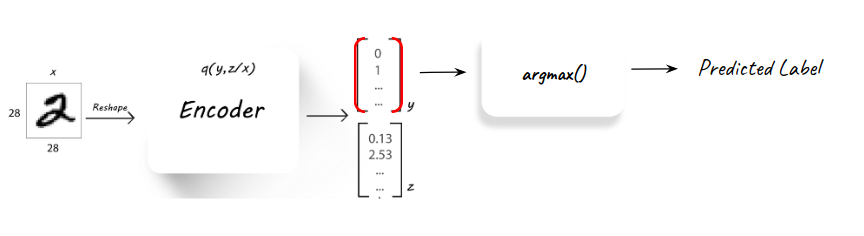
_images/adversarial_autoencoder_inference.png

This is how the model is tested and validated, using the inference process over a pre-known validation set.

The Training Process¶

The training process is divided into three major parts:

Auto Encoding (reconstruction) where the Encoder-Decoder networks (Q, P) learns to encode and reconstruct the image.
Adversarial where the encoder learns how to produce latent features y which are categorical and z which are normally distirbuted.
Semi-supervised where the encoder learns to predict the right label for a pre-known labeled image.

The success of the training process can be measured based on two grounds:

Validation accuracy on a held out labeled validation set. The results of the semi-supervised model reached 97% accuracy, which shows good performance and that the model learns the labeled part properly.

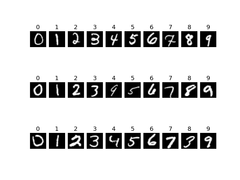
_images/semi_supervised_samples_from_all_lables.png

each column representing a predicted label for the original displayed images, showing the high accuracy of the model

Visual reconstruction Here we can see from visual examples that the reconstruction of an image (using the encoding-decoding pipeline) works pretty well. The reconstructed image is slightly blurry, which might be corrected with a slightly different loss function.

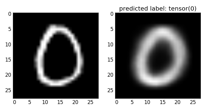
_images/semi_supervised_reconstruction_1.png

an example reconstruction of an original “0” digit image

In order to analyise the success of the adversarial part (which is focused on the latent features) we can examine the learning curve, showing the loss of the generator, and descriminator networks:

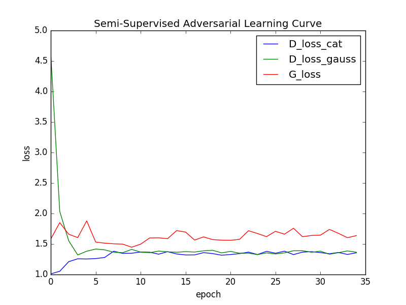
_images/semi_supervised_advesarial_learning_curve.png

the adversarial learning curve, showing the balance which is created between generator and discriminators

The Latent Features¶

The adverserial training pushes the latent features to the desired distribution. The latent y part learns to behave similarly to a categorial distribution, whlie the latent z part learns to distribute as a zero-centered normal.

First, we can see that the latent features were trained properly, using the adversarial balance.

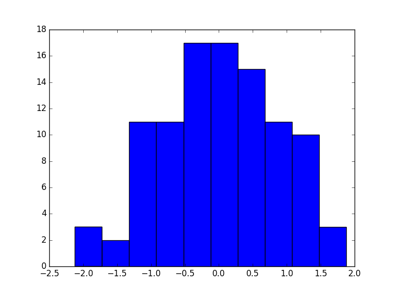
_images/semi_supervised_latent_z_distribution.png

the empricial distribution of the first dimension in the latent z vector, showing that the learned feature is indeed normally distributed around zero.

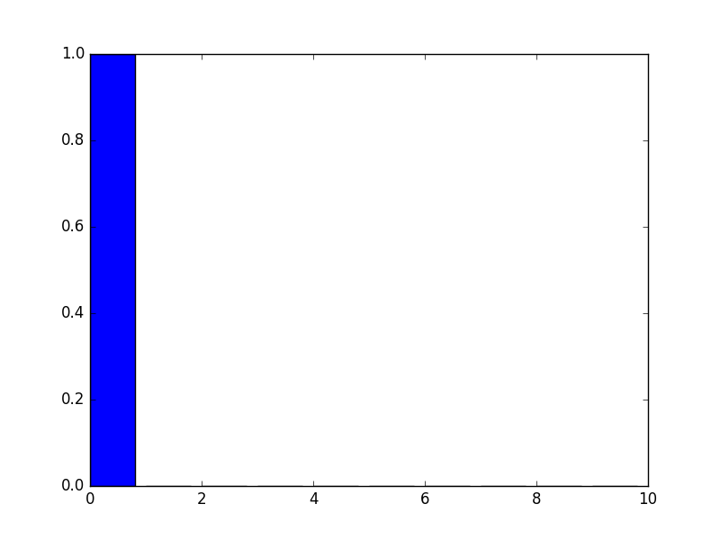
_images/semi_supervised_latent_y_example.png

an empricial example of the value of the latent y vector, showing that the learned feature is indeed categorial, showing close to “1” only near the predicted label.

Next we would like to find out if the latent features really perform as expected. The latent y vector is trained to learn the label, or “mode” of the input. We want it to describe the actual digit inside the input, and the semi-supervised procedure helps us reach that target.

The latent z vector is expected to represent “style”, and capture the deeper style of writing of a specific input digit. Again, this happens only thanks to the semi-supervision of known labels, pushing the latent y to capture what is neccesary to describe the type of digit.

Here’s a simple visualization of the meaning of the latent features:

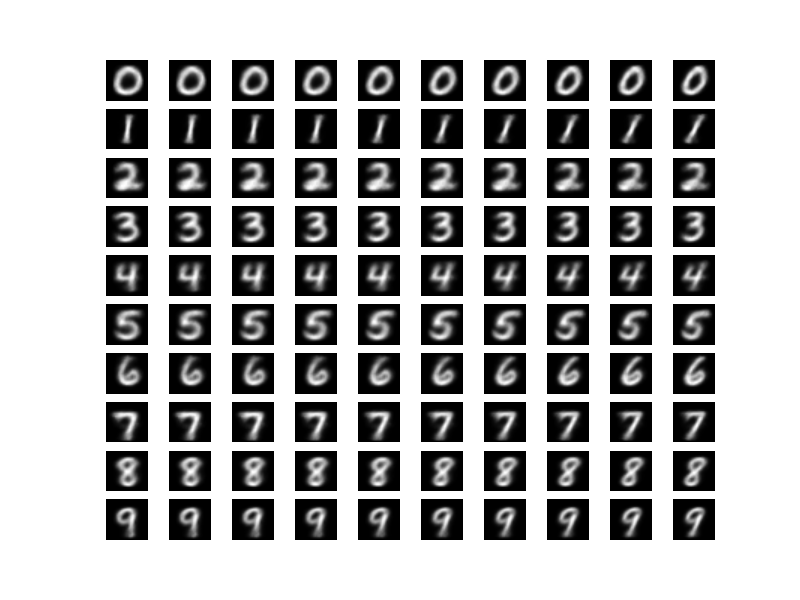
_images/semi_supervised_latent_features.png

each row represents a specific latent y value (out of the categorial distribution), and along that row the first dimension of the latent z vector is sampled uniformly from the normal distribution. One can see that indeed, the latent y completely catches the label, while the latent z controls the style and shape of the digit.

[1] A.Makhzani, J.Shlens, N.Jaitly, I.Goodfellow, B.Frey: Adversarial Autoencoders, 2016, arXiv:1511.05644v2