Initializing the Datasets
>>> python setup.py install --user
>>> init_datasets --dir-path <path-to-data-dir>
As a result the three datasets will be created in three different files inside the data directory: train_labeled.p, train_unlabeled.p, validation.p
Semi-supervised Training
>>> python setup.py install --user
>>> train_semi_supervised --dir-path <path-to-data-dir> --n-epochs 35 --z-size 2 --n-classes 10 --batch-size 100
As a result the following files will be created inside the data directory:
- Decoder / Encoder networks the Encoder-Decoder networks (Q, P) will be stored for future use and analysis under decoder_semi_supervised and encoder_semi_supervised
- Learning curves as png images, describing the adversarial, reconstruction and semi-supervised classification learning curves.
Un-supervised Training
>>> python setup.py install --user
>>> train_unsupervised --dir-path <path-to-data-dir> --n-epochs 35 --z-size 2 --n-classes 10 --batch-size 100
As a result the following files will be created inside the data directory:
- Decoder / Encoder networks the Encoder-Decoder networks (Q, P) will be stored for future use and analysis under decoder_unsupervised and encoder_unsupervised
- Mode Decoder network (if chosen in the configuration) responsible for the reconstruction of the image based on the categorial latent y, will be stored under mode_decoder_unsupervised
- Learning curves as png images, describing the adversarial, reconstruction and mutual information learning curves.
Visualization of the Learned Model
>>> python setup.py install --user
>>> generate_model_visualization --dir-path <path-to-data-dir> --model-dir-path {<path-to-model-dir> --mode unsupervised --n-classes 10 --z-size 5
As a result the following files will be created inside the model directory under a sub-directory called ‘visualization’:
- latent_features_tnse.png A 2-D visualization of the latent space using TSNE transformation over the validation set.
- learned_latent_features.png The role of the latent features over the reconstructed image.
- modes_and_samples_from_each_label.png Learned style-free modes of the Decoder model alongside real samples labeled by the AAE.
- predicted_label_distribution.png The distribution of the predicted labels.
- reconstruction_example.png An example of a real input and its reconstruction.
- y_distribution.png The distribution of the y latent space, representing a categorical distribution that can be used for labeling at inference. The plot shows the histogram of the maximum probability generated by the y latent vector.
- z_distribution.png The distribution of one of the nodes in the z latent vector.
- learned_modes.png In case of the Mode-Decoder being used as part of the model, this plot shows the modes learned by this decoder.
Hyperparmeter configuration
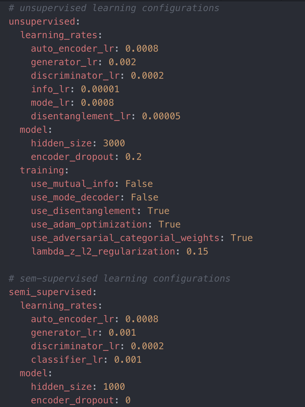
All hyper-paremeters are configurable via a YAML file. The only exclusions are the number of epochs, and the dimention of the latent z and y - which are all configurable via command line arguments when training the model.
The YAML configuration file contains many training and model configurations (as can be seen below) and in any training command the user can provide a path to the wanted config file. An example config file is found in the source code, and is used by default if another path is not provided.